Saturday, August 27, 2016

Designing heliostat layouts of concentrated solar power stations with Energy3D

Fig. 1: PS20 field output heat map (June, 22)
Fig. 2: PS20 field output heat map (December, 22)
Fig. 3: Fermat spiral layout (6/22, Phoenix, AZ)
In an earlier article, I have discussed the concepts and issues (shadowing, blocking, cosine efficiency, etc.) related to the design of heliostat layouts for concentrated solar power (CSP) tower stations. I also showed that these problems can be nicely visualized in Energy3D so that people can immediately see them. Instant visual feedback in design time may be very useful to a designer (in fact, this is known as concurrent analysis in the CAD/CFD community, meaning that the tasks of structure design and function simulation run immediately after each other to shorten the wait time between ideation and analysis). Figures 1 and 2 are the heat map visualizations of PS20, a CSP station in Spain, that instantly suggest the possibility of minor blocking problems for some heliostats in the summer and winter. The heat map on each reflector is based on the reflected portion of the direct solar radiation onto a 8 x 8 grid on the reflector plane. Hence it already includes shadowing loss, blocking loss, and attenuation loss. And you didn't read the image wrong, each heliostat reflector has a whopping area of 120 square meters (12 x 10 meters), dwarfing the vehicle in the image!

This blog post features several new tools that were just added to Energy3D to support the actual design tasks.

Fig. 4: Variations of layouts
The first tool is a field layout wizard that provides basic steps for customizing three different types of layout: circular, rectangular, and spiral. It allows you to select the width and height of the heliostat reflectors as well as a variety of parameters to automatically generate a layout. Of course, you can also easily copy and paste to create linear arrays of heliostats to create rectangular layouts. But the wizard does the job faster. Rectangular layouts can be seen at the Jülich Solar Tower in Germany and the Delingha Solar Tower in China. The latter just went into operation this August.

Note that, in Energy3D, the heliostat field must be built on top of a foundation. The size of the foundation you draw sets the boundary of the heliostat field. As the field layout must be done on a foundation, the layout wizard can only be accessed through the popup menu of a foundation.

The spiral layout that Energy3D supports (Figure 3) is an interesting addition. It currently provides the Fermat spiral, which is the pattern you see from a sunflower head. It is so amazing that solar science seems to always go back to the sunflower. The solar trackers for photovoltaic arrays mimic the motion of sunflowers to follow the sun. The spiral pattern of a sunflower head may hold a key to optimal heliostat layouts (Noone, Torrilhon, and Mitsos, Solar Energy, Vol. 862, pp. 792–803, 2012). This may not be too surprising considering that the sunflower has probably evolved into that particular pattern to ensure that each seed has enough room to grow and fair access to sunlight.

Fig. 5: Superimposed heliostats on top of map images (PS20)
The layout wizard provides a baseline model that you can always modify manually to get what you want (Figure 4). All heliostats can be easily dragged, dropped, or removed.

If you want to model after an existing CSP station, you can use the Geo-Location menu of Energy3D to import a map image of the station and then superimpose 3D heliostats on top of the map image where the images of the actual heliostats are located. Figure 5 shows that an Energy3D model of the PS20 station can be perfectly created using this method. The shadows on the ground cast by the heliostats in the Energy3D model even aligns very well with those captured in the map image (I must confess that I tried to guess the right date and time from the shadow of the tower and the rest just follows).

Thursday, August 25, 2016

Visualizing design issues in heliostat layouts of concentrated solar power stations with Energy3D

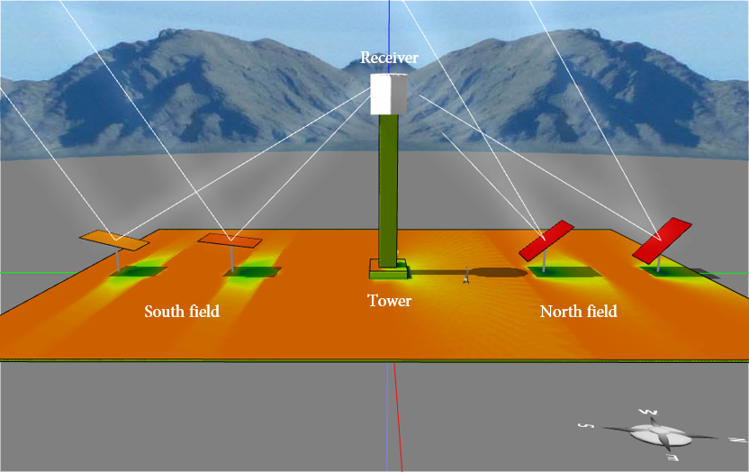
Fig. 1: Visualizing shadowing loss
As a one-stop-shop for solar solutions, Energy3D supports the design of concentrated solar power (CSP) stations. Although the main competitor of the CSP technology, the photovoltaic (PV) power stations, have become dominant in recent years due to the plummet of PV panel price, CSP has its own advantages and potential, especially in energy storage. According to the US Department of Energy, the levelized cost of electricity (LCOE) for CSP has dropped to 13 cents per kWh in the US in 2015, comparable to the LCOE for PV (12 cents per kWh). In general, it is always better to have options than having none. A combination of PV and CSP stations may be what is good for the world: CSP can complement PV to generate stable outputs and provide electricity at night. As a developer of solar design and simulation software, we are committed to supporting the research, development, and education of all forms of solar technologies.

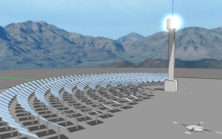
Numerical simulation plays an important role on designing optimal CSP stations. Concentrated solar power towers are the first type of CSP stations covered by the modeling engine of Energy3D. This blog post shows some progress towards the goal of eventually building a reliable simulation and visualization kernel for CSP tower technology in Energy3D. The progress is related to the study of heliostat layouts (the heat transfer part is yet to be built).

Numerous studies of heliostat layouts have been reported in literature in the past three decades, resulting in a variety of proposals for minimizing the land use and/or maximizing the energy output (see a recent review: Li, Coventry, Bader, Pye, & Lipiński, Optics Express, Vol. 24, No. 14, pp. A985-A1007, 2016). The latest is an interesting biomimetic pattern suggested by Noone, Torrilhon, and Mitsos (Solar Energy, Vol. 862, pp. 792–803, 2012), which resembles the spiral patterns of a sunflower head (each floret is oriented towards the next by the golden angle of 137.5°, forming a Fermat spiral that is probably Mother Nature's trick to ensure that each seed has enough room to grow and fair access to sunlight).

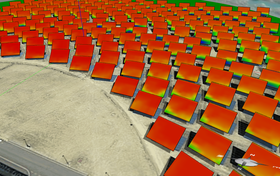
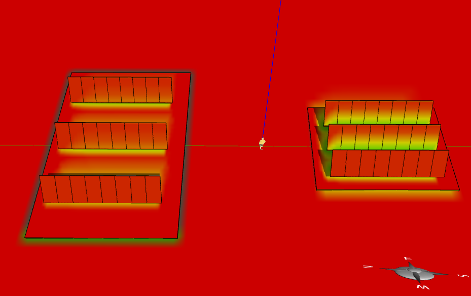
Fig. 2: Visualizing blocking loss
If you haven't worked in the field of solar engineering, you may be wondering why there has been such a quest for optimal layouts of heliostats. At first glance, the problem seems trivial -- well, a tower-based CSP station is just a gigantic solar cooker, isn't it? But things are not always what they seem.

The design of the heliostat layout is in fact a very complicated mathematical problem. We have some acres of land somewhere to begin with. The sun moves in the sky and its trajectory varies from day to day. But that is OK. The heliostats can be programmed to reflect sunlight to the receiver automatically. These all sound good until we realize that the heliostats' large reflectors can cast shadow to one another if they are too close or the sun is low in the sky (Figure 1). Like the case of PV arrays, shadowing causes productivity loss (but luckily, reflectors -- unlike solar panels based on strings of connected solar cells -- do not completely lose power if only a part of it is in the shadow).
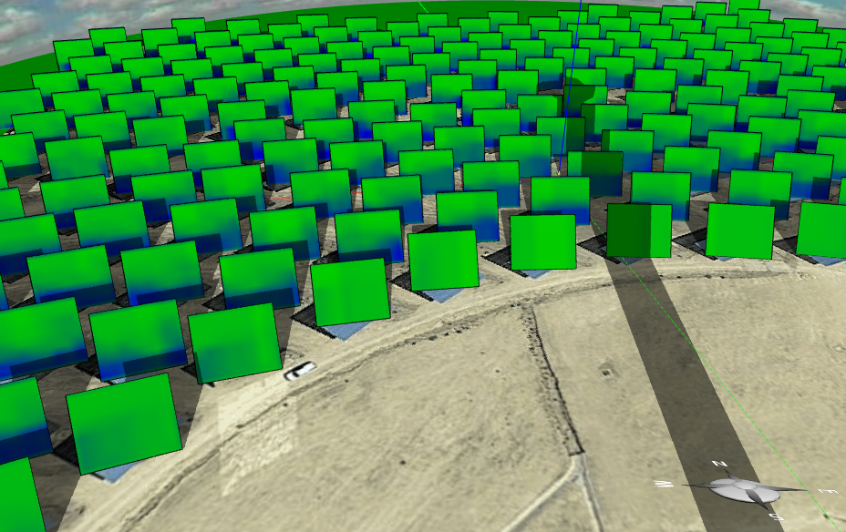
Fig. 3: Annual outputs of the heliostats in Fig. 2

Unlike the case of PV arrays, heliostats have an extra problem -- blocking. A heliostat must reflect the light to the receiver at the top of the tower and that path of light can be blocked by its neighbors. Of course, we rarely see the case of complete blocking. But if a portion of the reflector area is denied optical access to the receiver, the heliostat will lose some productivity. Energy3D can visualize this loss on each heliostat reflector. The upper image of Figure 2 shows the insolation to the reflectors whereas the lower one shows the portion of the insolation that actually reaches the receiver (you can see that the reflectors closer to the tower get more insolation). Figure 3 shows a comparison of the outputs of the heliostats over the course of a year. As you can see, the blue parts of the reflectors can never bounce light to the receiver because the heliostats in front of them block the reflection path for the lower parts of those heliostats. The way to mitigate this issue is to gradually increase the spacing between the heliostats when they are farther away from the tower.
Fig. 4: Visualizing cosine efficiency

Another problem with CSP tower technology is the so-called cosine efficiency. As we know, the insolation onto a surface is maximal when the surface directly faces the sun (this is known as the projection effect). In the northern hemisphere, however, the heliostats to the south of the tower (the south field) cannot face the sun directly as they must be positioned at an angle so that the incident sunlight can be reflected to a northern position (where the receiver is located). Figure 4 shows a visualization of the cosine effect and Figure 5 shows the comparison of the annual outputs of the heliostats. Clearly, the cosine efficiency is the lowest in the winter and the highest in the summer.
Fig. 5: Cosine efficiency is lower in the winter

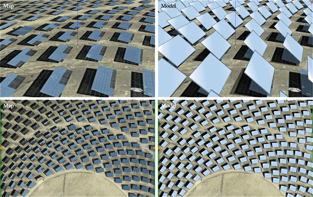
Does the cosine efficiency mean that we should only deploy heliostats in the north field as is shown in Figure 6? This depends on a number of factors. Yes, the cosine efficiency does reduce the output of a heliostat in the south field in the winter (maybe early spring and late fall, too), but a heliostat far away from the tower in the north field also produces less energy. For a utility-scale CSP station that must use thousands of heliostats, the part of the south field close to the tower may not be such a bad place to put heliostats, compared with the part of the north field far away from the tower. This is more so when the site is closer to the equator. If the site is at a higher latitude to the point that it makes more sense to deploy all heliostats in the north field, dividing the site into multiple areas and constructing a tower for each area may be a desirable solution. The downside is that additional towers will increase the constructional cost.
Fig. 6: Semicircular layout in the north field

We now multiply these three problems (shadowing, blocking, and cosine effect) with thousands of heliostats, confine them within an area of a given shape, and want to spend as less money as possible while producing as much electricity as possible. That is the essence of the mathematical challenge that we are facing in CSP field design. With even more functionalities to be added in the future, Energy3D could become a powerful design tool that anyone can use to search for their own solutions.

Wednesday, August 17, 2016

Choose solar trackers: HSAT, VSAT, or AADAT?

Fig. 1: HSAT and VSAT.
Energy3D now supports three major types of solar trackers: Horizontal single-axis trackers (HSAT), vertical single-axis trackers (VSAT), and altazimuth dual-axis trackers (AADAT). I have blogged about HSAT and AADAT earlier. Figure 1 shows the difference between HSAT and VSAT.

With all these options, which should we choose? The decision is based on the additional output of the solar panels, the space required to operate the system, and, of course, the cost of the tracking system. For instance, AADAT may be more complex as it rotates around two perpendicular axes. Space is always an important constraint and it is even more so for large solar farms considering the issue of inter-panel shading. Fixed arrays and HSAT systems may be more efficient in space usage if the inter-row shading is not significant.
Fig. 2 Energy3D predictions of annual outputs.

Let's first compare the annual output of a single solar panel under different conditions, as shown in Figure 2 and summarized in Table 1, calculated using Energy3D.

Table 1. Comparison of total annual outputs of a solar panel that has a fixed tilt angle equal to its latitude, a solar panel that is rotated by a HSAT, a solar panel that is rotated by a VSAT, and a solar panel that is rotated by an AADAT, at four different locations in the US. The unit is kWh.


Locations
Fixed (tilt=lat.)
HSAT
VSAT
AADAT
Boston, MA
428
520
559
603
Anchorage, AK
258
310
371
380
Miami, FL
507
654
617
711
San Juan, PR
523
694
617
738
 
These results suggest that the AADAT system, not surprisingly, generates the most electricity throughout the year at all four locations, as it always faces the sun. The second best, for low-latitude locations, is the HSAT system and, for high-latitude locations, is the VSAT system. In the case of HSAT, the lower the latitude, the closer the performance of the HSAT approaches that of the AADAT. In the case of VSAT, the higher the latitude, the closer the performance of the VSAT approaches that of the AADAT. This means that, considering the cost factor, HSAT at a very low latitude such as the equator is a better choice than AADAT and VSAT at a very high latitude such as Alaska is a better choice than AADAT.
Fig. 3 Optimal layout through heat map tessellation. 

The above analysis is based on a single, isolated solar panel. For arrays of panels, we must consider the shading area each panel sweeps when it is driven by a tracker. Energy3D's heat map visualization of solar irradiance may be a useful tool for designing optimal layouts for VSAT or AADAT panels that cannot be seamlessly aligned into rows such is in the case of HSAT arrays. From a mathematical point of view, an optimal layout must minimize land use. Hence, it can be imagined as a tessellation of effective shade area of individual panels (Figure 3). This may be something interesting to think about.

Friday, August 12, 2016

Simplifying solar design in Energy3D with Google Map integration

Fig. 1 2D view of Concord Consortium building in Energy3D
Solar design depends on accurate geometry. Rooftop solar panel design requires accurate 3D models of buildings, for example the shape of the roof, the height of the building, and the surrounding objects such as trees. Likewise, solar power station design requires accurate information about the field.

Fig. 2 3D view of Concord Consortium building in Energy3D
The easiest way to obtain these information is through Google Map, from which the dimension of an object can be measured. Although Google Map has not provided elevation data for a point yet, Google Earth does for many towns.

Earlier this year, students who performed solar design with Energy3D in our pilot tests must use Google Earth to retrieve the geometrical data for use in Energy3D design later. Having to master two sophisticated software tools simultaneously in a short time has turned out to be quite a challenge to many students. So an idea came to our mind: Why not just make Google Earth work within Energy3D? (Note: In fact, this is also a common feature among CAD software such as SketchUp.)

Fig. 3 Solar heat map of Concord Consortium building
It turned out that this integration is fairly simple, because Google has done the hard part of providing an easy-to-use Web API for virtually every platform. So in the latest version of Energy3D (V5.8.2 or higher), users will have an internal Google Map ready to help them with their solar designs.

Fig. 4 2D view of a solar farm in Concord, MA in Energy3D
Solar designers can specify a target location in Energy3D and then a Google Map image will be downloaded and used to overlay the ground in Energy3D. They can then draw a 3D building on top of this image by tracing the envelope of the building, eliminating the need to set the dimension of each side numerically. Figures 1-3 demonstrate the result of this new feature using the Concord Consortium's office building as an example.

Fig. 5 3D view of a solar farm in Concord, MA in Energy3D
A remarkable advantage brought by this feature is that it is easy to add model trees on top of the images of surrounding trees. A future version will also allow users to adjust the height and spread of a model tree based on the Google Map image.

Other than assisting designers to acquire site data, the map image also provides a rendering of how a new design may look like in an environment with existing buildings (just pretend for a moment that the building in Figure 2 hadn't existed and were a proposal to build two new houses at the site). Furthermore, with Google Map's elevation API, we will also be able to construct a terrain model of the ground (which is currently flat). Such a terrain model will not only make the energy simulation more accurate by taking all the surrounding objects into account but also make the rendering more realistic by giving the 2D map image a 3D effect (similar to the new 3D view of Google Map).

Based on Energy3D, we have created two solar design challenges for students to make meaningful contributions to the solarization movement. One is to solarize their own houses by designing rooftop solar panels. The other is to solarize their own schools and towns by designing solar farms (Figures 4 and 5). Aligned with the Next Generation Science Standards (NGSS) that require students to think and act like scientists and engineers, our goal is to engage students to practice science and engineering through solving real-world problems. But real-world problems are often complex and difficult (otherwise they are not problems in the real world!). This calls for the development of advanced tools that can empower students to tackle real-world problems. Our Energy3D software provides examples of how technology may knock down the barriers and help students attain the high standards set by the NGSS.

Friday, August 5, 2016

Modeling horizontal single-axis solar trackers in Energy3D

In the last post, I have blogged about modeling dual-axis solar trackers in Energy3D. To be more precise, the trackers shown in that blog post are altitude-azimuth (Alt/Az), or altazimuth trackers, or AADAT in short. In this post, I will introduce a type of single-axis tracker -- the horizontal single-axis tracker, or HSAT in short.

Fig. 1 Solar panel arrays rotated by HSATs
Because single-axis trackers do not need to follow the sun exactly, there are many different designs. Most of them differ in the choice of the axis of rotation. If the axis is horizontal to the ground, the tracker is a HSAT. If the axis is vertical to the ground, the tracker is a vertical single-axis tracker, or VSAT in short. All trackers with axes of rotation between horizontal and vertical are considered tilted single-axis trackers, or TSAT in short. None of these single-axis trackers can help the solar panels capture 100% of the solar radiation that reaches the ground. Exactly which design to choose depends on the location of the solar farm, among other consideration such as the cost of the mechanical system.

Fig. 2 Compare daily outputs of HSAT, AADAT, and fixed in four seasons.
HSAT is the first type of single-axis tracker that has been implemented in Energy3D. HSAT is probably more common than VSAT and TSAT and is probably easier to construct and install. In most cases, the rotation axis of a HSAT aligns with the north-south direction and the solar panels follow the sun in an east-to-west trajectory, as is shown in the YouTube video embedded in this post and in Figure 1.

Fig. 3 Compare annual outputs of HSAT, AADAT, and fixed.
How much more energy can a HSAT help to generate? Figure 2 shows the comparison of the outputs of a HSAT system, an AADAT system, and an optimally fixed solar panel on March 22, June 22, September 22, and December 22, respectively, in the Boston area. The results suggest that the HSAT system is almost as good as the AADAT system in June but its performance declines in March and September and becomes the worst in December (in which case it can only capture a little more than half of the energy harvested by the AADAT system). Interestingly, also notice that there is a dip at noon in the energy graphs for March, September, and December. Why so? I will leave the question for you to figure out. If you have a hard time imagining this, perhaps the visualizations in Energy3D can help.

Fig. 4 Compare wide- and narrow-spacing of HSAT arrays
Figure 3 shows the annual result, which suggests that, over the course of a year, the HSAT system -- despite of its relatively unsatisfactory performance in spring, fall, and winter -- still outperforms any fixed solar panel, but it captures about 86% of the energy captured by the AADAT system.

An important factor to consider in solar farm design is the choice of the inter-row spacing to avoid significant energy loss due to shading of adjacent rows in early morning and late afternoon. But you don't want the distance between two rows to be too far as the rows will occupy a large land area that makes no economic sense. With Energy3D, we can easily investigate the change of the energy output with regard to the change of the inter-row spacing. Figure 4 shows the gain from HSAT is greatly reduced when the rows are too close, essentially eliminating the advantages of using solar trackers. Despite of their ability to track the sun, HSATs still require space to achieve the optimal performance.