Wednesday, July 26, 2017

Thermal imaging as a universal indicator of chemical reactions: An example of acid-base titration

Fig. 1: NaOH-HCl titration
Funded by the National Science Foundation, we are exploring the feasibility of using thermal imaging as a universal indicator of chemical reactions. The central tenet is that, as all chemical reactions absorb or release thermal energy (endothermic or exothermic), we can infer certain information from the time evolution and spatial distribution of the temperature field.

To prove the concept, we first chose titration, a common laboratory method of quantitative chemical analysis that is used to determine the unknown concentration of an identified analyte, as a beginning example. A reagent, called the titrant, is prepared as a standard solution. A known concentration and volume of titrant reacts with a solution of analyte to determine its concentration.

The experiment we did today was an acid-base titration. An acid–base titration is the determination of the concentration of an acid or base by exactly neutralizing the acid or base with a base or acid of known concentration. Such a titration is typically done with a burette that drops titrant into an Erlenmeyer flask containing the analyte. A pH indicator is used to determine whether the equivalence point has been reached. The pH indicator usually depends on the analyte and the titrant. But a differential thermal analysis based on infrared imaging may provide a universal indicator as the technique depends only on the heat of reaction and thermal energy is universal.

Fig. 2: The dish-array titration revealed by FLIR ONE
Figures 1 and 2 in this article show the results of the NaOH+HCl titration, taken using a FLIR ONE thermal camera attached to my iPhone 6. A solution of 10% NaOH was prepared as the analyte of "unknown" concentration and 1%, 3%, 5%, 7%, 10%, 12%, 15%, 18%, and 20% HCl were used as the titrant. The experiment was conducted with a 3×3 array of Petri dishes. Hence, we call this setup as dish-array titration. Preliminary results of this first experiment appeared to be encouraging, but we have to be cautious as the dissolving of HCl after the acid-base neutralization completes can also release a significant amount of heat. How to separate the thermal signatures of reaction and dissolving requires some further thinking.

Thursday, July 20, 2017

Analyzing the linear Fresnel reflectors of the Sundt solar power plant in Tuscon

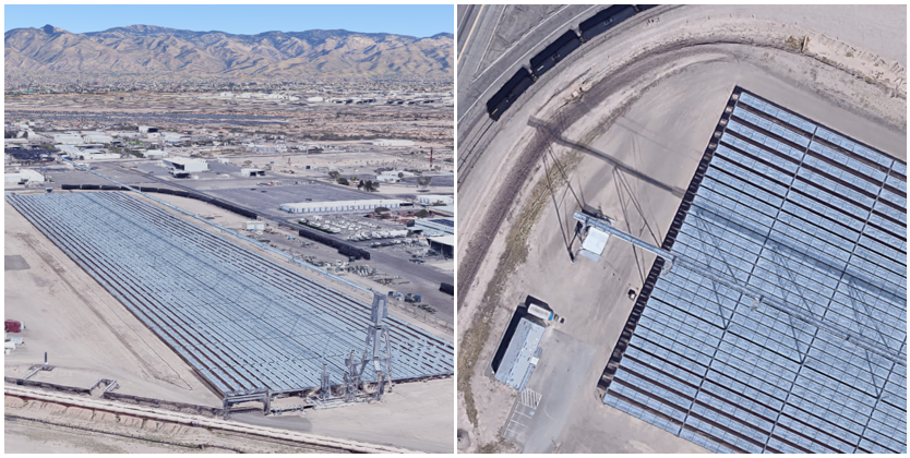
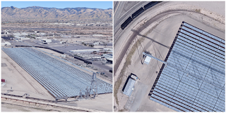
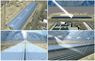
Fig. 1: The Sundt solar power plant in Tuscon, AZ
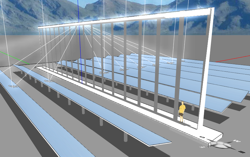
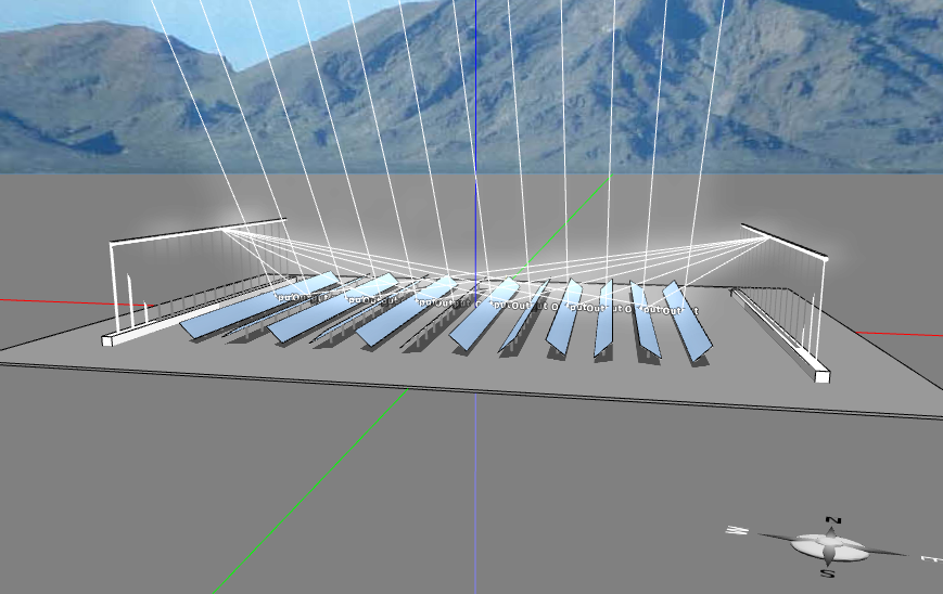
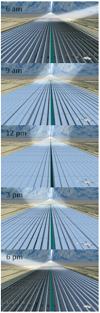
Fig. 2: Visualization of incident and reflecting light beams
Tucson Electric Power (TEP) and AREVA Solar constructed a 5 MW compact linear Fresnel reflector (CLFR) solar steam generator at TEP’s H. Wilson Sundt Generating Station -- not far from the famous Pima Air and Space Museum. The land-efficient, cost-effective CLFR technology uses rows of flat mirrors to reflect sunlight onto a linear absorber tube, in which water flows through, mounted above the mirror field. The concentrated sunlight boils the water in the tube, generating high-pressure, superheated steam for the Sundt Generating Station. The Sundt CLFR array is relatively small, so I chose it as an example to demonstrate how Energy3D can be used to design, simulate, and analyze this type of solar power plant. This article will show you how various analytic tools built in Energy3D can be used to understand a design principle and evaluate a design choice.
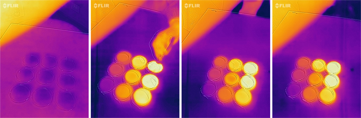
Fig. 3: Snapshots
One of the "strange" things that I noticed from the Google Maps of the power station (the right image in Figure 1) is that the absorber tube stretches out a bit at the northern edge of the reflector assemblies, whereas it doesn't at the southern edge. The reason that the absorber tube was designed in such a way becomes evident when we turn on the light beam visualization in Energy3D (Figure 2). As the sun rays tend to come from the south in the northern hemisphere, the focal point on the absorber tube shifts towards the north. During most days of the year, the shift decreases when the sun rises from the east to the zenith position at noon and increases when the sun lowers as it sets to the west. This shift would have resulted in what I call the edge losses if the absorber tube had not extended to the north to allow for the capture of some of the light energy bounced off the reflectors near the northern edge. This biased shift becomes less necessary for sites closer to the equator.

Energy3D has a way to "run the sun" for the selected day, creating a nice animation that shows exactly how the reflectors turn to bend the sun rays to the absorber pipe above them. Figure 3 shows five snapshots of the reflector array at 6am, 9am, 12pm, 3pm, and 6pm, respectively, on June 22 (the longest day of the year).

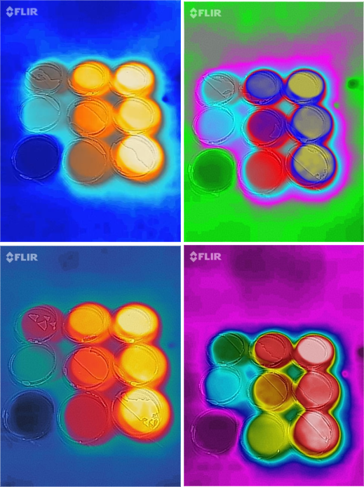
As we run the radiation simulation, the shadowing and blocking losses of the reflectors can be vividly visualized with the heat map (Figure 4). Unlike the heat maps for photovoltaic solar panels that show all the solar energy that hits them, the heat maps for reflectors show only the reflected portion (you can choose to show all the incident energy as well, but that is not the default).

There are several design parameters you can explore with Energy3D, such as the inter-row spacing between adjacent rows of reflectors. One of the key questions for CLFR design is: At what height should the absorber tube be installed? We can imagine that a taller absorber is more favorable as it reduces shadowing and blocking losses. The problem, however, is that, the taller the absorber is, the more it costs to build and maintain. It is probably also not very safe if it stands too tall without sufficient reinforcements. So let's do a simulation to get in the ballpark. Figure 5 shows the relationship between the daily output and the absorber height. As you can see, at six meters tall, the performance of the CLFR array is severely limited. As the absorber is elevated, the output increases but the relative gain decreases. Based on the graph, I would probably choose a value around 24 meters if I were the designer.
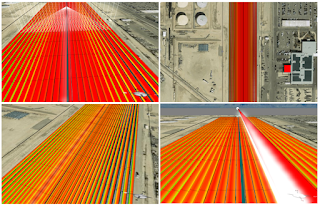
Fig. 4: Heat map visualization

An interesting pattern to notice from Figure 5 is a plateau (even a slight dip) around noon in the case of 6, 12, and 18 meters, as opposed to the cases of 24 and 30 meters in which the output clearly peaks at noon. The disappearance of the plateau or dip in the middle of the output curve indicates that the output of the array is probably approaching the limit.

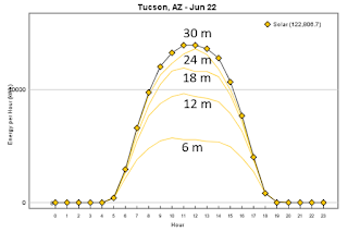
Fig. 5: Daily output vs. absorber height
If the height of the absorber is constrained, another way to boost the output is to increase the inter-row distance gradually as the row moves away from the absorber position. But this will require more land. Engineers are always confronted with this kind of trade-offs. Exactly which solution is the optimal depends on comprehensive analysis of the specific case. This level of analysis used to be a professional's job, but with Energy3D, anyone can do it now.

Saturday, July 15, 2017

Modeling linear Fresnel reflectors in Energy3D

Fig. 1: Fresnel reflectors in Energy3D.
Fig. 2: An array of linear Fresnel reflectors
Linear Fresnel reflectors use long assemblies of flat mirrors to focus sunlight onto fixed absorber pipes located above them, thus capable of concentrating sunlight to as high as 30 times of its original intensity (Figures 1 and 2). This concentrated light energy is then converted into thermal energy to heat a fluid in the pipe to a very high temperature. The hot fluid gives off the heat through a heat exchanger to power a steam generator, like in other concentrated solar power plants such as parabolic troughs and power towers.

Fig. 3: Heap map view of reflector gains
Compared with parabolic troughs and power towers, linear Fresnel reflectors may be less efficient in generating electricity, but they may be cheaper to build. According to Wikipedia and the National Renewable Energy Laboratory, Fresnel reflectors are the third most used solar thermal technology after parabolic troughs and power towers, with about 15 plants in operation or under construction around the world. To move one small step closer to our goal of providing everyone a one-stop-shop solar modeling software program for solarizing the world, I have added the design, simulation, and analysis capabilities of this type of concentrated solar power technology in Version 7.1.8 of Energy3D.

Fig. 4: Compact linear Fresnel reflectors.
Fig. 5: Heat map view of linear Fresnel reflectors for two absorber pipes.
Like parabolic troughs, Fresnel reflectors are usually aligned in the north-south axis and rotate about the axis during the day for maximal efficiency (interestingly enough, however, some of the current Fresnel plants I found on Google Maps do not stick to this rule -- I couldn't help wondering the rationale behind their design choices). Unlike parabolic troughs, however, the reflectors hardly face the sun directly, as they have to bounce sunlight to the absorber pipe. The reflectors to the east of the absorber start the day with a nearly horizontal orientation and then gradually turn to face west. Conversely, those to the west of the absorber start the day with an angle that faces east and then gradually turn towards the horizontal direction. Due to the cosine efficiency similar to the optics related to heliostats for power towers, the reflectors to the east collect less energy in the morning than in the afternoon and those to the west collect more energy in the morning and less in the afternoon.

Like heliostats for power towers, Fresnel reflectors have both shadowing and blocking losses (Figure 3). Shadowing losses occur when a part of a reflector is shadowed by another. Blocking losses occur when a part of a reflector that receives sunlight cannot reflect the light to the absorber due to the obstruction of another reflector. In addition, Fresnel reflectors suffer from edge losses -- the focal line segments of certain portions near the edges may fall out of the absorber tube and their energy be lost, especially when the sun is low in the sky. In the current version of Energy3D, edge losses have not been calculated (they are relatively small compared with shadowing and blocking losses).

Linear Fresnel reflectors can focus light on multiple absorbers. Figure 4 shows a configuration of a compact linear Fresnel reflector with two absorber pipes, positioned to the east and west of the reflector arrays, respectively. With two absorber pipes, the reflectors may be overall closer to the absorbers, but the downside is increased blocking losses for each reflector (Figure 5).

Wednesday, July 12, 2017

Simulation-based analysis of parabolic trough solar power plants around the world

Fig. 1: 3D heat map of the Keahole Plant in Hawaii
Fig. 2: SEGS-8 in California and NOOR-1 in Morocco
In Version 7.1.7 of Energy3D, I have added the basic functionality needed to perform simulation-based analysis of solar power plants using parabolic trough arrays. These tools include 24-hour yield analysis for any selected day, 12-month annual yield analysis, and the 3D heat map visualization of the solar field for daily shading analysis (Figure 1). The heat map representation makes it easy to examine where and how the design can be optimized at a fine-grained level. For instance, the heat map in Figure 1 illustrates some degree of inter-row shadowing in the densely-packed Keahole Solar Power Plant in Hawaii (also known as Holaniku). If you are curious, you can also add a tree in the middle of the array to check out its effect (most solar power plants are in open space with no external obstruction to sunlight, so this is just for pure experimental fun).
Fig. 3: Hourly outputs near Tuscon in four seasons

Fig. 4: Hourly outputs near Calgary in four seasons
As of July 12, I have constructed the Energy3D models for nine such solar power plants in Canada, India, Italy, Morocco, and the United States (Arizona, California, Florida, Hawaii, and Nevada) using the newly-built user interface for creating and editing large-scale parabolic trough arrays (Figure 2). This interface aims to support anyone, be she a high school student or a professional engineer or a layperson interested in solar energy, to design this kind of solar power plant very quickly. The nine examples should sufficiently demonstrate Energy3D's capability of and relevance in designing realistic solar power plants of this type. More plants will be added in the future as we make progress in our Solarize Your World Initiative that aims to engage everyone to explore, model, and design renewable energy solutions for a sustainable world.
Fig. 5: Hourly outputs near Honolulu in four seasons

An interesting result is that the output of parabolic troughs actually dips a bit at noon in some months of the year (Figure 3), especially at high altitudes and in the winter, such as Medicine Hat in Canada at a latitude of about 51 degrees (Figure 4). This is surprising as we perceive noon as the warmest time of the day. But this effect has been observed in a real solar farm in Cary, North Carolina that uses horizontal single-axis trackers (HSATs) to turn photovoltaic solar panels. Although I don't currently have operation data from solar farms using parabolic troughs, HSAT-driven photovoltaic solar arrays that align in the north-south axis work in a way similar to parabolic troughs. So it is reasonable to expect that the outputs from parabolic troughs should exhibit similar patterns. This also seems to agree with the graphs in Figure 6 of a research paper by Italian scientists that compares parabolic troughs and Fresnel reflectors.

The effect is so counter-intuitive that folks call it "Solar Array Surprises." It occurs only in solar farms driven by HSATs (fixed arrays do not show this effect). As both the sun and the solar collectors move in HSAT solar arrays, exactly how this happens may not be easy to imagine at once. Some people suggested that the temperature effect on solar cell efficiency might be a possible cause. Although it is true that the decrease of solar cell efficiency at noon when temperature rises to unfavorable levels in the summer of North Carolina can contribute to the dip, the theory cannot explain why the effect is also pronounced in other seasons. But Energy3D accurately predicts these surprises, as I have written in an article about a year before when I added supports for solar trackers to Energy3D. I will think about this more carefully and provide the explanation later in an article dedicated to this particular topic. For now, I would like to point out that Energy3D shows that the effect diminishes for sites closer to the equator (Figure 5).

Friday, July 7, 2017

Designing panda solar power plants with Energy3D

Fig. 1: Panda power in Energy3D
Fig. 2: Panda power in Energy3D
A Panda-shaped photovoltaic (PV) solar power plant in Datong, China recently came online and quickly went viral in the news. While solar power plants in cute shapes are not a new thing (I blogged about the Mickey Mouse-shaped solar farm in Orlando, FL about six weeks ago), this one drew a lot of attentions because the company that built it, Panda Green Energy Group, is reportedly planning to build 100 more such plants around the world to advertise for renewable energy. According to the company's website, the idea of building Panda-shaped solar power plants originated from Ada Li, a student from Oregon Episcopal School. Li proposed her idea at the COP21 Conference in Paris.

The construction of the 100 MW Datong Panda Solar Power Plant began on November 20, 2016. It is expected to generate 3.2 billion KWh in a life span of 25 years. The plant consists of two types of solar panels of different colors: black monocrystalline solar panels and white thin-film solar panels. The two types form the characteristic shape and pattern of a giant panda, the national treasure of China and the logo of the World Wildlife Fund. Considering the number of people who complain about solar power plants being eyesores in their neighborhoods, these attempts by the Panda and Micky Mouse solar farms and their future cousins may provide examples to mitigate these negative perceptions.

Fig. 3: A close-up view of Panda power.
Fig. 4: A close-up view of Panda power.
One of our summer interns, Maya Haigis, who is a student from the University of Rochester, spent a couple of hours to create an Energy3D model of the Datong Panda Solar Power Plant after I shared the news with her today. The power plant is so new that Google Maps currently show only a picture of it under construction. So Maya went ahead to draw the power plant based on an artist's imagination taken from the news. Her design ended up using about 34,000 solar panels. To make it look like a real giant panda with its trademark black and white fur, I had to quickly add a light gray color option for solar panels in Energy3D. Maya's work came out to be amazingly realistic (Figures 1 and 2). This is even more remarkable considering that Maya had no prior experience with Energy3D.

Panda Green Energy said in the press release that they designed the power plant also for the purpose of engaging youth to join the renewable energy revolution. They are planning to reach out to schools for student site visits. There is also a plan to make the power plant a tourist attraction. I am not sure people would pay to go there to see it. But with Energy3D, we can imagine the experience by taking a virtual tour with the 3D model (Figures 3 and 4). The engineers among us can run Energy3D simulations to analyze its performance and investigate whether such an effort makes scientific sense.

So what about inviting children all over the world to "paint" the brownfields that have scarred our planet with this kind of good-looking solar power plants using Energy3D as a "solar brush?" Welcome to our Solarize Your World Initiative!

Thursday, July 6, 2017

Energy3D turns the globe into a powerful engineering design lab for everyone

Fig. 1: Dots represent regions supported in Energy3D.
Many of the readers of my blog may not know Energy3D is, in fact, also a Google Maps application. Energy3D allows users to import a satellite image of a site through the Google Maps API as the "ground image" in its 3D coordinate system, on top of which users can draw 3D structures such as buildings or power plants. Built-in simulation engines can then be used to test and analyze these structures without having to switch to another tool and leave the scene (something known as "concurrent analysis" in the CAD industry). These engines use large geographical and weather datasets for the site as inputs for simulations to accurately take environmental factors such as air temperature and solar radiation into account. As the climate is probably the single most important factor that drives the energy usage in buildings where we live and work, it is important to use weather data from a typical meteorological year (TMY) in a simulation. If no weather data is available for the site, Energy3D will automatically select the nearest location from a network of more than 525 supported worldwide regions (Figure 1) when you import the satellite image from Google Maps. The following table lists the numbers of regions in 176 countries that are currently supported in Energy3D. The United States is covered by a network of 164 nodes. So if you are in the United States, you will have a better chance to find a location that may represent the climate of your area.

Afghanistan 1 Albania 1 Algeria 6
Angola 1 Argentina 3 Armenia 1
Australia 11 Austria 1 Azerbaijan 1
Bahamas 1 Bahrain 1 Bangladesh 1
Belarus 1 Belgium 1 Belize 1
Bolivia 1 Bosnia & Herzegovina 1 Botswana 1
Brazil 8 Brunei 1 Bulgaria 1
Burkina Faso 1 Burundi 1 Cambodia 1
Cameroon 1 Canada 10 Cape Verde 1
Central African Republic 1 Chad 1 Chile 12
China 42 Colombia 2 Comoros 1
Congo 1 Costa Rica 1 Croatia 1
Cuba 1 Cyprus 2 Czech 1
DR Congo 1 Denmark 1 Djibouti 1
Dominica 1 Dominican Republic 1 East Timor 1
Ecuador 1 Egypt 1 El Salvador 1
Equatorial Guinea 1 Eritrea 1 Estonia 1
Ethiopia 1 Fiji 2 Finland 1
France 8 Gabon 1 Gambia 1
Georgia 1 Germany 12 Ghana 1
Greece 2 Guatemala 1 Guinea 1
Guinea-Bissau 1 Guyana 1 Haiti 1
Honduras 1 Hungary 1 Iceland 1
India 11 Indonesia 4 Iran 3
Iraq 1 Ireland 1 Israel 1
Italy 5 Ivory Coast 1 Jamaica 1
Japan 6 Jerusalem 1 Jordan 1
Kazakhstan 1 Kenya 1 Kosovo 1
Kuwait 1 Kyrgyzstan 1 Laos 1
Latvia 1 Lebanon 1 Lesotho 1
Liberia 1 Libya 2 Liechtenstein 1
Lithuania 1 Luxembourg 1 Macedonia 1
Madagascar 1 Malawi 1 Malaysia 2
Maldives 1 Mali 1 Malta 1
Marshall Islands 1 Mauritania 1 Mauritius 1
Mexico 4 Moldova 1 Monaco 1
Mongolia 1 Montenegro 1 Morocco 3
Mozambique 1 Myanmar 2 Namibia 1
Nepal 1 Netherlands 1 New Zealand 2
Nicaragua 1 Niger 1 Nigeria 1
North Korea 1 Norway 1 Oman 1
Pakistan 4 Panama 1 Papua New Guinea 1
Paraguay 1 Peru 2 Philippines 1
Poland 7 Portugal 2 Qatar 1
Republic of China 2 Romania 1 Russia 7
Rwanda 1 Saudi Arabia 2 Senegal 1
Serbia 2 Sierra Leone 1 Singapore 1
Slovakia 1 Slovenia 1 Solomon Islands 1
Somalia 1 South Africa 8 South Korea 2
South Pole 1 South Sudan 1 Spain 8
Sri Lanka 1 Sudan 1 Sweden 1
Switzerland 3 Syria 2 Tajikistan 1
Tanzania 2 Thailand 2 Togo 1
Trinidad & Tobago 1 Tunisia 1 Turkey 3
Turkmenistan 1 Uganda 1 Ukraine 2
United Arab Emirates 2 United Kingdom 6 United States 164
Uruguay 1 Uzbekistan 1 Venezuela 1
Vietnam 2 Western Sahara 1 Yemen 1
Zambia 1 Zimbabwe 1

Fig. 2: Solar sites in Fitchburg, MA.
Energy3D's capability of turning Google Maps into a gigantic virtual engineering design lab has tremendous potential in STEM education and energy revolution. It allows students to pick and choose sites for designing renewable energy and energy efficiency solutions that are most relevant to their lives, such as their home and school buildings (Figure 2). It gives students an authentic tool that supports them to scientifically investigate all sorts of possibilities to design a more sustainable world and effectively communicate their ideas to the public. And, most importantly, with Energy3D being a free tool that anyone can use at zero cost, this can happen at the global scale to engage every student in the world to act now and make a difference!

This global vision is not new. Back in 1995, the National Science Foundation funded my colleagues Boris Berenfeld, Bob Tinker, and Dan Barstow, who were at TERC at that time, a grant to develop a curriculum that they touted as the Globe Lab. The Global Lab Curriculum meant to provide an interdisciplinary, one-year course at the secondary level that supports science standards and school reform through intercultural, scientifically meaningful, and collaborative student investigations in environmental studies. Students were given the opportunity to experience all aspects of genuine scientific research: problem identification, background study, project design, collaboration, data analysis, and communication.

Fig. 3: Solar power plants around the world.
More than 20 years later, technology has advanced so much that we now have many more resources and tools to rethink about this idea. With Google Maps and weather data for countless regions in the world, Energy3D is poised to become a true example of Globe Lab for science and engineering. The integration of the software and our Solarize Your World Curriculum with the current, unstoppable waves of renewable energy innovation and movement worldwide will create numerous exciting possibilities for youth to become truly involved and engaged in shaping their world and their future (Figure 3). While we undertake this grand challenge, it is utterly important to keep in mind that renewable energy does not just stand for some kind of green ideology related only to potential tax hikes -- it also represents trillions of dollars worth of business opportunities and investment in the coming decades committed by almost all governments on the planet to revamp the world's energy infrastructure to provide cleaner air and healthier environment for their citizens. Given this level of global significance, our work will only become more essential and the implications will only become more profound.

As we are mourning the loss of Bob Tinker, one of the architects of the Global Lab Curriculum, carrying on this line of work will be the best way to remember his visions, honor his contributions, and celebrate his life.